Why Your Excel PivotTable Still Misses New Rows After Refresh
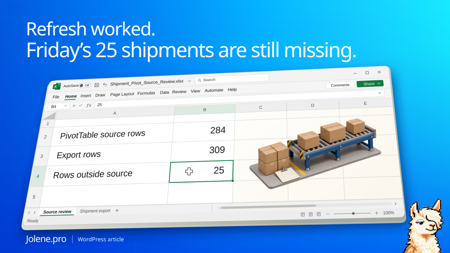
Friday’s shipment rows are in the workbook. You hit Refresh and the dashboard remains at 284 shipments. The PivotTable is still reading the same fixed range, which ends a row before the first Friday entry.
Open Change Data Source and compare its last row with the export. If the report uses a fixed cell range, point it at an Excel Table that includes all the current rows and refresh again.
Find the break between the export and the PivotTable
This export has one shipment per row and headers in row 1.
| Check | Old source | Complete source |
|---|---|---|
| Range | A1:F285 | A1:F310 |
| Records | 284 | 309 |
| Last shipment | S-1284 | S-1309 |
The source range missed 25 rows. The PivotTable wasn’t failing to refresh. It was refreshing the same 284 records.
Recreate the 25 missing shipments
In a blank Excel desktop workbook, name a sheet Shipments. Paste this tab-separated block into A1. It creates six headers and the first synthetic record:
ShipmentID	ShipDate	Carrier	Lane	Status	Units
="S-"&(ROW()+999)	=IF(ROW()<=285,DATE(2026,11,12),DATE(2026,11,13))	DemoCarrier	Local	Shipped	1
Select A2:F310 and use Home → Fill → Down to copy row 2 through row 310. Format B2:B310 as dates. Keep this layout unchanged during the exercise; the formulas use row numbers. English function names and comma separators are shown; your Excel locale may require semicolons.
Create a standard worksheet PivotTable with the source explicitly set to Shipments!$A$1:$F$285. Put Carrier in Rows and ShipmentID in Values, summarized by Count. Leave all filters and slicers clear. The expected count is 284, even though the sheet contains 309 shipment IDs. This example deliberately counts IDs, with one unique, nonblank ID per shipment.
Check A285: it should be S-1284. The first omitted ID is S-1285 in A286, and the last is S-1309 in A310. Their dates in B286:B310 are all Friday, November 13, 2026. The old range contains Thursday’s November 12 records only.
On this blank practice sheet, use =COUNTA(A2:A285) for the old-source control of 284 and =COUNTA(A2:A310) for the full-source control of 309. The omitted block =COUNTA(A286:A310) must equal 25. These controls assume the generated IDs have no blanks or duplicates.
Change the PivotTable source to Shipments!$A$1:$F$310 and refresh it. The expected count is now 309. For the reusable version, convert A1:F310 to an Excel Table named ShipmentLog, change the PivotTable source to ShipmentLog and refresh. Creating a table nearby does not by itself prove the existing PivotTable now uses it. Reopen Change Data Source and verify the table name.
Inspect what the PivotTable is actually connected to
Click inside the PivotTable and check its data source. For a fixed worksheet range, compare its final row to the report’s last stable ID. If it is connected to Power Query or the Data Model, inspect that query or connection instead.
Create a source that expands with the file
Select the full records and create an Excel Table with unique headers. Change the source to the table and append future rows inside it or directly below it, checking that the table expanded. After refreshing, look for slicers or filters that can still hide the new records.
Check a stale and a current snapshot together
Keep a copy of what the report actually included, plus the latest export. This makes it straightforward to distinguish missing records from a filter or date issue.
Which shipment IDs are present in the latest export but absent from the source used in the report? Show the first missing row, affected dates and source cells.
Record the 309-row check in the refresh notes. Next Friday, check the last shipment ID again before distributing the dashboard.
For an ordinary worksheet total beside a filtered list, use the separate visible-row SUBTOTAL exercise. It shows why a $1,200 visible subtotal can coexist with a $1,500 East branch balance.
Microsoft on PivotTable sources · Microsoft on refreshing PivotTables
The figures and identifiers in this example are synthetic.
The record counts, ID sequence and dates above were independently checked. Native Excel PivotTable creation and refresh were not performed during this check, and a live Jolene.pro result could not be verified. These are expected results for a synthetic exercise.
Microsoft documents how to change the PivotTable source and use an Excel Table as the source. If the rows are included but the report counts invoice amounts rather than adding them, use the separate Count versus Sum practice guide. Find more examples in Jolene.pro Workbook Studies.
Try this with your own spreadsheet at Jolene.pro. Follow Jolene.pro on LinkedIn for more spreadsheet guides.
3 comments