How to Sum Only Visible Rows After Filtering in Excel
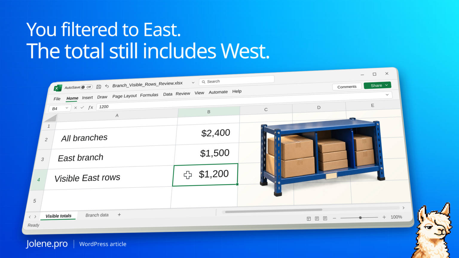
You filter the collections worksheet to the East branch and copy the total into a follow-up email. The figure still includes the West branch. The filter changed which invoices you can see while SUM kept adding the same range.
Use SUBTOTAL with function number 109 for a sum that skips filtered-out and manually hidden rows. Check which rows you mean to include before using the visible total in a report.
The rows visible in the collection list
This sample is filtered to East. One East invoice row has also been hidden manually.
| Invoice | Branch | Balance | Display state |
|---|---|---|---|
| INV-501 | East | $1,200 | Visible |
| INV-502 | West | $900 | Filtered out |
| INV-503 | East | $300 | Hidden manually |
SUM across the three cells returns $2,400. SUBTOTAL with 9 returns $1,500. SUBTOTAL with 109 returns $1,200. The right number depends on whether the manually hidden row should count.
Reproduce the three totals in specific cells
On a blank Excel desktop worksheet, paste the following tab-separated data into A1. Enter the balances as numbers, without a currency symbol:
Invoice	Branch	Balance
INV-501	East	1200
INV-502	West	900
INV-503	East	300
Keep the following control formulas below the data rows, so hiding row 4 will not hide the controls. Put their labels in E6:E9 and the formulas in F6:F9:
| Cell | Label | Formula |
|---|---|---|
| F6 | All invoices | =SUM(C2:C4) |
| F7 | Filtered subtotal, including manually hidden rows | =SUBTOTAL(9,C2:C4) |
| F8 | Visible-row subtotal | =SUBTOTAL(109,C2:C4) |
| F9 | East branch balance | =SUMIFS(C2:C4,B2:B4,B2) |
Select only A1:C4 and turn on Data → Filter. First leave every invoice visible. Then filter Branch to East. Finally, while that filter remains active, hide worksheet row 4 using its row header. INV-503 is the manually hidden East invoice; INV-502 in row 3 is excluded by the branch filter.
| Worksheet state | SUM | SUBTOTAL 9 | SUBTOTAL 109 | SUMIFS East |
|---|---|---|---|---|
| All three rows visible | $2,400 | $2,400 | $2,400 | $1,500 |
| East filter only | $2,400 | $1,500 | $1,500 | $1,500 |
| East filter and row 4 hidden manually | $2,400 | $1,500 | $1,200 | $1,500 |
The $300 gap between F7 and F8 is INV-503 at C4. Hiding that invoice does not remove its balance from East’s receivables. Use F9 for the stated East-only business rule; use F8 for the visible-row snapshot and label it accordingly. To reset the exercise, unhide row 4 and clear the branch filter.
Use the right SUBTOTAL function number
Place the formula outside the Balance data range so it doesn’t include itself. Filtered-out rows are excluded by both versions. Function 9 includes manually hidden rows, and 109 skips them.
=SUBTOTAL(109,C2:C4)Check the scope independently
If you want East regardless of how the sheet is filtered, calculate that business rule explicitly with SUMIFS. Keep a date and filter record when exporting the visible subtotal. A screenshot alone can miss hidden rows that affect a calculation.
Trace the totals to an explicit branch list
Give the review an explicit branch, status or date rule. If workbook display state is relevant, record that state or use a separate visible-row extract.
Reconcile the all-branch balance with the East branch list and identify the exact invoice rows included under the stated rule.
Label the reported figure clearly. East outstanding balance and visible-row subtotal can legitimately differ.
Microsoft SUBTOTAL reference · Microsoft on summing by multiple conditions
The figures and identifiers in this example are synthetic.
The amounts and included-row sets above were independently calculated using Microsoft’s documented SUBTOTAL rules. Native Excel filtering, hiding and recalculation were not performed during this check, and a live Jolene.pro result could not be verified. These are expected synthetic results.
Keep this exercise’s balance data in one vertical column, with no nested subtotal rows. Formula examples use English names and comma separators; some Excel locales require semicolons. If a report omits new records even after refresh, the separate PivotTable source-range exercise checks that problem. Browse more practice material in Jolene.pro Workbook Studies.
Try this with your own spreadsheet at Jolene.pro. Follow Jolene.pro on LinkedIn for more spreadsheet guides.
1 comment